Tutorial (MATLAB)

Here is an example shows how to use OCEANLYZ. In this example, we use a provided sample file “waterpressure_5burst.csv” as input data. This sample file contains five bursts of water pressure data recorded with a pressure sensor. Sample file may be downloaded at akarimp/oceanlyz .

Measurement properties for “waterpressure_5burst.csv” are:

Properties	Value	OCEANLYZ Properties
File name	waterpressure_5burst.csv
Data type	Water pressure (Pa)	obj.InputType=’pressure’
Number of recorded burst (n_burst)	5	obj.n_burst=5
Sampling frequency (fs)	10 (Hz)	obj.fs=10
Recording duration (burst_duration)	1024 (second)	obj.burst_duration=1024
Pressure sensor height from bed (heightfrombed)	0.05 (m)	obj.heightfrombed=0.05
Mean water depth (h)	Varies in each burst

To start using OCEANLYZ, first, we need to be in a folder that contains OCEANLYZ files. Assume OCEANLYZ files are in ‘C:\oceanlyz_matlab’. First, we change current working directory to OCEANLYZ folder as:

cd('C:\oceanlyz_matlab') %Change current working directory to OCEANLYZ folder

Next, we download water pressure dataset (“waterpressure_5burst.csv”), we unzip it and copy sample files in a desired folder.

Assume we are currently in OCEANLYZ folder ‘C:\oceanlyz_matlab’ and downloaded sample data file is stored in ‘C:\oceanlyz_matlab\Sample_Data’. Then, we load data as:

current_folder = pwd;                %Current (OCEANLYZ) path
cd('C:\oceanlyz_matlab\Sample_Data') %Change current folder to a folder that contains data file
water_pressure = importdata('waterpressure_5burst.csv'); %Load data
cd(current_folder)                   %Change current folder back to initial (OCEANLYZ) folder

We can plot data if we need to as:

plot(water_pressure)
xlabel('Sample points')
ylabel('Water Pressure (N/m^2)')

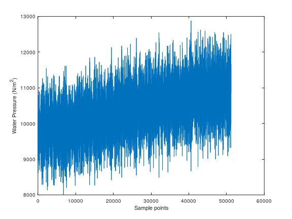
Figure 1: Plot of input water pressure data

Then, we need to create an OCEANLYZ object as:

%Create OCEANLYZ object
ocn = oceanlyz;

Next, we assign wave data to OCEANLYZ object as:

%Input data
ocn.data = water_pressure;

Now, we set up OCEANLYZ properties as:

ocn.InputType='pressure';
ocn.OutputType='wave+waterlevel';
ocn.AnalysisMethod='spectral';
ocn.n_burst=5;
ocn.burst_duration=1024;
ocn.fs=10;
ocn.fmin=0.05;
ocn.fmax=ocn.fs/2;
ocn.fmaxpcorrCalcMethod='auto';   %Only required if ocn.InputType='pressure'
ocn.Kpafterfmaxpcorr='constant';  %Only required if ocn.InputType='pressure'
ocn.fminpcorr=0.15;               %Only required if ocn.InputType='pressure'
ocn.fmaxpcorr=0.55;               %Only required if ocn.InputType='pressure'
ocn.heightfrombed=0.05;           %Only required if ocn.InputType='pressure'
ocn.dispout='yes';
ocn.Rho=1024;                     %Seawater density (Varies)

After all required properties are set, we can run OCEANLYZ as:

ocn.runoceanlyz()

Output is stored as a structure array. Name of output is ‘oceanlyz_object.wave’. Field(s) in this structure array can be called by using ‘.’ For example oceanlyz_object.wave.Hm0 contains zero-moment wave height and oceanlyz_object.wave.Tp contains peak wave period.

Here we show how to plot zero-moment wave height:

Hm0 = ocn.wave.Hm0; %zero-moment wave height
plot(Hm0)
xlabel('Burst Number')
ylabel('Hm0 (m)')

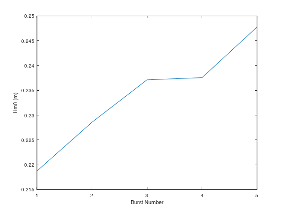
Figure 2: Plot of \(H_{m0}\) versus burst number

Similarly, we can plot wave spectrum for the first burst:

f = ocn.wave.f; %frequency of the first burst
Syy = ocn.wave.Syy; %spectrum of the first burst
plot(f(1,:),Syy(1,:))
xlabel('f (Hz)')
ylabel('Syy (m^2/Hz)')

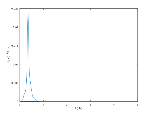
Figure 3: Plot of \(S_{yy}\) versus f

Notes

Note1:

If data are collected in continuous mode and you need to analyze them in smaller blocks, you can analyze it in a burst mode. For that, you choose n_burst and burst_duration as follow:

The burst_duration is equal to a period of time that you want data analyzed over that. For example, if you need wave properties reported every 15 min, then the burst_duration would be 15*60 second.

the n_burst is equal to the total length of the time series divided by the burst_duration. The n_burst should be an integer. So, if the total length of the time series divided by the burst_duration leads to a decimal number, then data should be shortened to avoid that.

Note2:

Welch spectrum is used to calculate a power spectral density. In all spectral calculation, a default window function with a default overlap window between segments are used.

Note3:

If fmaxpcorrCalcMethod=’auto’, then OCEANLYZ calculates fmaxpcorr based on water depth and a sensor height from a seabed (refer to Applying Pressure Response Factor section). A maximum value for calculated fmaxpcorr will be limited to the value user set for fmaxpcorr.